

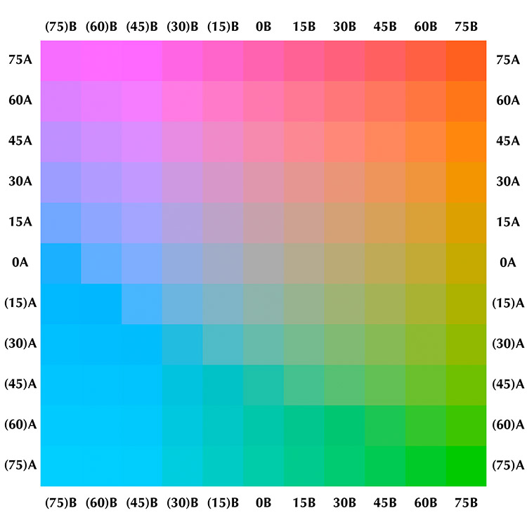
For those interested in how LAB works, and also in gamut issues, I’ve posted a downloadable LAB grid for experimentation. It looks, more or less, like this:
For posting, this graphic has been converted to sRGB, but you can download the LAB original for experiments.
The vertical axis, from top to bottom, goes from positive to negative in the A channel, that is, from magenta to teal. The horizontal axis, from left to right, goes from negative to positive in the B, or from blue to yellow. The maximum value is +75 and the minimum -75; the grid is in 15-point increments. The very center point of the grid is therefore 0a0b, a neutral.
When you open the file, the L value is a constant 70L, where 100L is pure lightness and 0L pure darkness. However, a curves adjustment layer allows you to change the L to whatever you like. Interesting things happen when you do.
For example, in the right-hand column of the center row, the current value is 70L0a75b. LAB theory says that this is a brilliant yellow, but as we can see, it’s more of a golden shade.
This happens because there’s no such thing as a yellow this dark. If we lighten the grid to, say, 85L, then the yellowness becomes apparent. But if we do that, we will no longer recognize the upper right corner as being red. In fact, even as it stands the upper right is more of an orange than a red. We’d have to crank up the L channel to say, 50L before we’d see what could be called deep reds.
The other major use of this tool is to evaluate gamut. Inexperienced users sometimes try to force more color into an LAB file than the output device can take. When this happens, usually detail gets lost and the color doesn’t improve.
LAB is supposed to be “perceptually uniform”, which for present purposes means that each square in the grid should be just as distinct against its neighbors as any square elsewhere on the grid would be. As you can see, that certainly isn’t true in the lower left corner, the rich cyans; definitely the squares are more distinct higher up in the grid.
What you are looking at now isn’t an LAB file, because the site can’t display one. Instead, I converted it to sRGB for posting. The lower left calls for colors that are out of the sRGB gamut, so everything kind of got smooshed together. That’s how I know that you can’t see the distinctions: they’re actually missing from the file you’re viewing. Here’s a graphic that illustrates the differences between the sRGB file and what the LAB file calls for. Where the background is light gray, there is no difference. Elsewhere, the bigger the difference, the more intensely it shows up in the graphic, and clearly the biggest differences are in the lower left.

This graphic shows what gets lost when the basic LAB grid gets converted into sRGB. The light gray background indicates no change, meaning that the LAB file called for something within the sRGB gamut. In other areas, the more intense the color, the farther out of gamut was the LAB original.
In the downloadable file, though, the distinctions are there. The question is whether you will be able to see them on your screen. The more important question is whether you will be able to see them if you attempt to print the file. And then you may need to consider what happens if you change the grid’s L value, which will cause other squares to become less distinct even if, perhaps, it restores the distinctions in the lower left.
If you like to push the envelope on colors, these questions can become important. All systems of calibration have trouble at the edges of the gamut. Now matter how well calibrated you think your system is, there’s no guarantee that all your devices will agree in these tricky areas. A member of the appliedcolortheory list tried an interesting experiment: he viewed the LAB file on several different monitors, including some that are designed for high-end production, a laptop, and a monitor not ordinarily used to view pictures. To his surprise, he reported that the squares were more distinct on the inferior monitors.
I hope you find the download interesting.
{ 20 comments… read them below or add one }
Thanks Dan, fascinating AND useful – what more could we ask!
A suggestion: on my wish list for future PPW revisions, is a button for the Apply Image command. I’m using it a great deal & as I use 2 27″ monitors, one for palettes etc & one for the image my hand does a lot of travelling. THis would be great.
Aroha, not everyone uses two monitors ;-).
In early versions of the panel there was in fact an Apply Image button. We removed it on the grounds that we really wanted to save space and that it wasn’t efficient. Apply Image always requires that we move the cursor away from the panel to its dialog. It’s therefore quicker to assign a keyboard shortcut to Apply Image and navigate to the dialog rather than moving to the panel, finding the button and clicking it, and then going to the dialog.
Note that this objection doesn’t apply to the Convert to LAB/RGB buttons, which could also theoretically be removed. Click one of those, and the next click will be in the panel, or we will invoke a keyboard shortcut, but we won’t have to cut across to another dialog.
Dear master, it is a pleasure to contact you. I am brazilian, and I am reading your book on color corrections on your PPW system. In chapter 3 of the book, page 49, you used the terms “blow out” and “plug”. I’m having difficulty fully understand what these words mean. Would be to give me a synonym or clarify the idea!
Valter,
If Portuguese behaves like Italian and Spanish then I would translate “blown out” as “luzes queimadas”. I don’t know of a precise synonym for “plugged” so I would say “uma perda de detalhes nas sombras”
The two concepts are the same in that they both describe a failure to retain detail, but they are the opposite in that one refers to the lightest areas of the image and the other to the darkest areas.
I wish that the translators of my books would ask questions like this when they run across phrases that they don’t understand!
Ok Master,
Grateful for the prompt reply, so I think I understand correctly. I believe the correct term in Portuguese (Brazil), would “estourar” (burst), which means a specular light (the color of the paper) and the other “clipping”, black with no detail.
Thanks for your attention!
Dear Master,
When I downloaded the images to study in chapter 3, the images of hockey players were not present, Is there some problem to release this image? I ask this because I would have them for a note in detail of what is described in the book. Another doubt I have is; how to run the files “.acv” (curves) that came along with the images?
Valter,
The hockey image is included in the chapter 3 download package. The file name is Ch03 Fig 3-12 hockey-sm. It is downsized from the book size by request of the owner, but this does not affect your ability to practice with it.
To load the curves, click the small flyout box to the right of the Preset field at the top of the Curves dialog. Then choose Load Preset and Photoshop will ask you for the location of the .acv you wish to load.
Dear Master,
A tip on how to download the curves were perfectly clear, and worked well, but the same did not happen with the file “CH03 Fig 3-12 sm-hockey.” I managed to download it to my PC, however, it does not run. All other files have the extension JPEG, this has no extension. The Photosho CS6 can not open it and inform in your box “Could not complete your request because it is not the right kind of document”. When I tried to open it in using Windows, the application also can not run it, opens a box in there to try to find a program that can run it. So the conclusion is that either the file is corrupt or was improperly saved on your server. Being impossible to run it. Just for the avoidance of doubt, both my Windows as my Photoshop were purchased legally along with their manufacturers, both Microsoft and Adobe. If the case be hard to solve the problem, no problem, because I ended up using the techniques taught here in another kind of photo. But I’m telling you it, because maybe some other reader has the same problem occurred. A hug. I hope you had a good Easter!
Thanks,
Valter,
Just add the .jpg suffix manually, and then the file should open.
The best solutions are always the simplest. It worked perfectly. Thanks!
Just for the register, in the book “Modern Photoshop Color Workflow” page 59, there is an error in the exercise box below. In the last question, the item number 5, it says “The dark sweater in Figure 3.17E.” the correct would be “The dark sweater in Figure 3.17D.” The Figure 3.17E is a picture of some people kidding on the beach, have nothing with dark sweater. I Hope to have helped!
Thanks for sharing information about calibration tool, it was awesome post. I believe that this information helps in implementation of as per calibration services .
Valter, Thanks for trying to help, but you read the question incorrectly. It is not “the dark sweater” but “the dark seawater” (a água escura do mar) and Figure 3.17E is the correct reference.
Ok, I understand, was my fault. I hit the color, but missed in translation.
However, I have a other doubt. In the text p.64 is described “Assuring color fidelity in objects that are about deleted, such as gray card, is a low priority. Assuming you agree that exaggerated colors of Figure 3.21B are superior to those of 3.21A, you have just decided that an inaccurate gray card is acceptable.”
I think that the ideia not stayed clear. It would not be ” Assuring color fidelity in objects that are about to be deleted, such as a gray card is a low priority. Assuming you agree that the exaggerated colors of Figure 3.21B are better than 3.21A, what we realize is that even an inaccurate assessment of gray is acceptable to the fix the color balance. The original idea is not to despise the evaluation of the gray card and seek a review by the internal evidence of the image?
Forgive me if I seem boring, but understand the idea for me is very important, without fully understanding the concept the reading is becoming increasingly difficult.
Hi Dan,
thanks for sharing this great LAB grid. Do you know why the positive “a” values are nearly everywhere mentioned as red (and not magenta)? I found that very misleading in other publications. As far as I have read about LAB, you are the only author who refers positive a as magenta and not red.
Best Regards,
Martin
Oh Martin,
This is really a constant detail in the speech of Master Dan, but more importantly I think about everything I have seen so far, is the easy which Mr. Margulis can pass the numeric range for color variation, both in LAB as for RGB. This is fantastic! Understanding these changes is support for all the work to fix.
Martin,
Up until the turn of the century *everyone* referred to the A channel as red-green; I did so myself in the first two editions of Professional Photoshop (1993 and 1997).
By the end of the century I was spending more time studying LAB and I realized that “red-green” was inaccurate. I was the first to call it “magenta-green”, in Professional Photoshop Third Edition (aka Professional Photoshop 6) in 2000. Today we still find sources that have picked up the obsolete “red-green” but anybody who’s serious about working in LAB now won’t use that term.
I thought hard about calling it magenta-teal rather than magenta-green, because a value of A-negative B-zero is much too blue for vegetation, yet not blue enough to warrant calling the color cyan. But anyone expecting that the leaves of trees would be this color might have a nasty surprise.
I decided to just stick with “green” because “teal”, although fairly accurate, may not be familiar to everyone, particularly those whose first language is not English. “Magenta”, meanwhile, is a word that everyone understands, and everyone who looks at LAB understands that an A-positive B-zero value is magenta, not red.
Dan and Valter,
thanks for your answers. Dan, I think you are right concerning the word “teal” for people whose first language isn’t english. As a non native speaker, I had to consult an online dictionary for the meaning of teal.
Concerning this red vs. magenta thoughts, I made my own chart. You can download it here, if you are interested : http://giebel-foto.de/download/Lab-rot-Diagramm.jpg
It shows a-values from 0 to max (x-axis) in steps of L by increasing 10 each (y-axis). You can find hues that I would suggest as red, but the great majority is clearly magenta. Thanks for the discussion folks.
Best Regards from germany,
Martin
Not trying to be rude I have tried three times to subscribe to the 10 hrs of free videos but never get a return email
Thank you
Don,
The response is automated, so it must be being intercepted, presumably by a spam filter. So first, check your spam folders. If this doesn’t work, our troubleshooting page is here.